Introduction to pandas#
Note
This material is mostly adapted from the following resources:

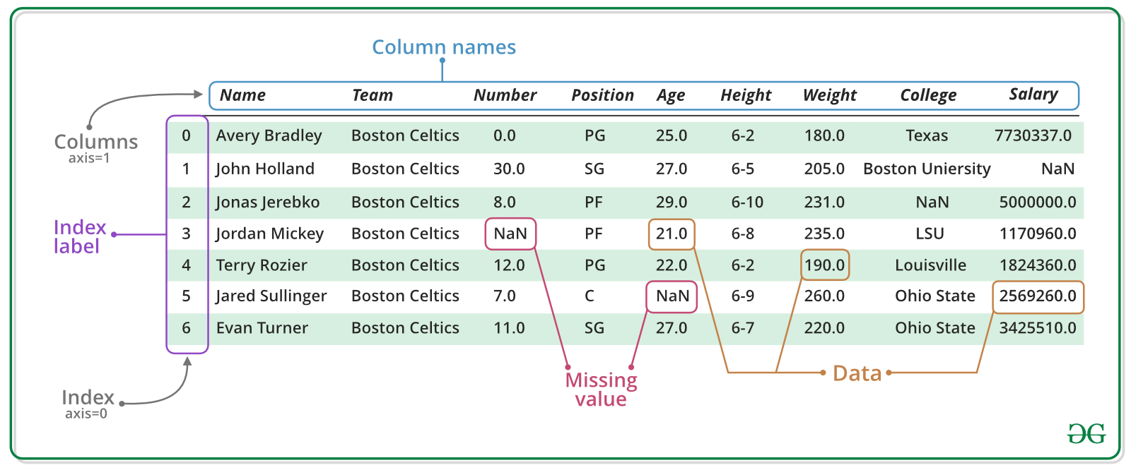
Pandas is a an open source library providing high-performance, easy-to-use data structures and data analysis tools. Pandas is particularly suited to the analysis of tabular data, i.e. data that can can go into a table. In other words, if you can imagine the data in an Excel spreadsheet, then Pandas is the tool for the job.
A fast and efficient DataFrame object for data manipulation with indexing;
Tools for reading and writing data: CSV and text files, Excel, SQL;
Intelligent data alignment and integrated handling of missing data;
Flexible reshaping and pivoting of data sets;
Intelligent label-based slicing, indexing, and subsetting of large data sets;
High performance aggregating, merging, joining or transforming data;
Hierarchical indexing provides an intuitive way of working with high-dimensional data;
Time series-functionality: date-based indexing, frequency conversion, moving windows, date shifting and lagging;
Note
Documentation for this package is available at https://pandas.pydata.org/docs/.
Note
If you have not yet set up Python on your computer, you can execute this tutorial in your browser via Google Colab. Click on the rocket in the top right corner and launch “Colab”. If that doesn’t work download the .ipynb file and import it in Google Colab.
Then install pandas and numpy by executing the following command in a Jupyter cell at the top of the notebook.
!pip install pandas numpy
import pandas as pd
import numpy as np
Pandas Data Structures: Series#
A Series represents a one-dimensional array of data. The main difference between a Series and numpy array is that a Series has an index. The index contains the labels that we use to access the data.
There are many ways to create a Series. We will just show a few. The core constructor is pd.Series().
(Data are from Wikipedia’s List of power stations in Germany.)
names = ["Neckarwestheim", "Isar 2", "Emsland"]
values = [1269, 1365, 1290]
s = pd.Series(values, index=names)
s
Neckarwestheim    1269
Isar 2            1365
Emsland           1290
dtype: int64
dictionary = {
    "Neckarwestheim": 1269,
    "Isar 2": 1365,
    "Emsland": 1290,
}
s = pd.Series(dictionary)
s
Neckarwestheim    1269
Isar 2            1365
Emsland           1290
dtype: int64
Arithmetic operations and most numpy functions can be applied to pd.Series.
An important point is that the Series keep their index during such operations.
np.log(s) / s**0.5
Neckarwestheim    0.200600
Isar 2            0.195391
Emsland           0.199418
dtype: float64
We can access the underlying index object if we need to:
s.index
Index(['Neckarwestheim', 'Isar 2', 'Emsland'], dtype='object')
We can get values back out using the index via the .loc attribute
s.loc["Isar 2"]
1365
Or by raw position using .iloc
s.iloc[2]
1290
We can pass a list or array to loc to get multiple rows back:
s.loc[["Neckarwestheim", "Emsland"]]
Neckarwestheim    1269
Emsland           1290
dtype: int64
And we can even use slice notation
s.loc["Neckarwestheim":"Emsland"]
Neckarwestheim    1269
Isar 2            1365
Emsland           1290
dtype: int64
s.iloc[:2]
Neckarwestheim    1269
Isar 2            1365
dtype: int64
If we need to, we can always get the raw data back out as well
s.values # a numpy array
array([1269, 1365, 1290])
Pandas Data Structures: DataFrame#
There is a lot more to Series, but they are limit to a single column. A more useful Pandas data structure is the DataFrame. A DataFrame is basically a bunch of series that share the same index. It’s a lot like a table in a spreadsheet.
The core constructor is pd.DataFrame()
Below we create a DataFrame.
# first we create a dictionary
data = {
    "capacity": [1269, 1365, 1290],  # MW
    "type": ["PWR", "PWR", "PWR"],
    "start_year": [1989, 1988, 1988],
    "end_year": [np.nan, np.nan, np.nan],
}
df = pd.DataFrame(data, index=["Neckarwestheim", "Isar 2", "Emsland"])
df
| capacity | type | start_year | end_year | |
|---|---|---|---|---|
| Neckarwestheim | 1269 | PWR | 1989 | NaN |
| Isar 2 | 1365 | PWR | 1988 | NaN |
| Emsland | 1290 | PWR | 1988 | NaN |
We can also switch columns and rows very easily.
df.T
| Neckarwestheim | Isar 2 | Emsland | |
|---|---|---|---|
| capacity | 1269 | 1365 | 1290 |
| type | PWR | PWR | PWR |
| start_year | 1989 | 1988 | 1988 |
| end_year | NaN | NaN | NaN |
A wide range of statistical functions are available on both Series and DataFrames.
df.min()
capacity      1269
type           PWR
start_year    1988
end_year       NaN
dtype: object
df.mean(numeric_only=True)
capacity      1308.000000
start_year    1988.333333
end_year              NaN
dtype: float64
df.std(numeric_only=True)
capacity      50.467812
start_year     0.577350
end_year            NaN
dtype: float64
df.describe()
| capacity | start_year | end_year | |
|---|---|---|---|
| count | 3.000000 | 3.000000 | 0.0 |
| mean | 1308.000000 | 1988.333333 | NaN |
| std | 50.467812 | 0.577350 | NaN |
| min | 1269.000000 | 1988.000000 | NaN |
| 25% | 1279.500000 | 1988.000000 | NaN |
| 50% | 1290.000000 | 1988.000000 | NaN |
| 75% | 1327.500000 | 1988.500000 | NaN |
| max | 1365.000000 | 1989.000000 | NaN |
We can get a single column as a Series using python’s getitem syntax on the DataFrame object.
df["capacity"]
Neckarwestheim    1269
Isar 2            1365
Emsland           1290
Name: capacity, dtype: int64
…or using attribute syntax.
df.capacity
Neckarwestheim    1269
Isar 2            1365
Emsland           1290
Name: capacity, dtype: int64
Indexing works very similar to series
df.loc["Emsland"]
capacity      1290
type           PWR
start_year    1988
end_year       NaN
Name: Emsland, dtype: object
df.iloc[2]
capacity      1290
type           PWR
start_year    1988
end_year       NaN
Name: Emsland, dtype: object
But we can also specify the column(s) and row(s) we want to access
df.loc["Emsland", "start_year"]
1988
df.loc[["Emsland", "Neckarwestheim"], ["start_year", "end_year"]]
| start_year | end_year | |
|---|---|---|
| Emsland | 1988 | NaN |
| Neckarwestheim | 1989 | NaN |
df.capacity * 0.8
Neckarwestheim    1015.2
Isar 2            1092.0
Emsland           1032.0
Name: capacity, dtype: float64
Which we can easily add as another column to the DataFrame:
df["reduced_capacity"] = df.capacity * 0.8
df
| capacity | type | start_year | end_year | reduced_capacity | |
|---|---|---|---|---|---|
| Neckarwestheim | 1269 | PWR | 1989 | NaN | 1015.2 |
| Isar 2 | 1365 | PWR | 1988 | NaN | 1092.0 |
| Emsland | 1290 | PWR | 1988 | NaN | 1032.0 |
We can also remove columns or rows from a DataFrame:
df.drop("reduced_capacity", axis="columns")
| capacity | type | start_year | end_year | |
|---|---|---|---|---|
| Neckarwestheim | 1269 | PWR | 1989 | NaN |
| Isar 2 | 1365 | PWR | 1988 | NaN |
| Emsland | 1290 | PWR | 1988 | NaN |
We can update the variable df by either overwriting df or passing an inplace keyword:
df.drop("reduced_capacity", axis="columns", inplace=True)
We can also drop columns with only NaN values
df.dropna(axis=1)
| capacity | type | start_year | |
|---|---|---|---|
| Neckarwestheim | 1269 | PWR | 1989 |
| Isar 2 | 1365 | PWR | 1988 |
| Emsland | 1290 | PWR | 1988 |
Or fill it up with default “fallback” data:
df.fillna(2023)
| capacity | type | start_year | end_year | |
|---|---|---|---|---|
| Neckarwestheim | 1269 | PWR | 1989 | 2023.0 |
| Isar 2 | 1365 | PWR | 1988 | 2023.0 |
| Emsland | 1290 | PWR | 1988 | 2023.0 |
Say, we already have one value for end_year and want to fill up the missing data:
df.loc["Emsland", "end_year"] = 2023
# backward (upwards) fill from non-nan values
df.fillna(method="bfill")
/tmp/ipykernel_2116/532230991.py:2: FutureWarning: DataFrame.fillna with 'method' is deprecated and will raise in a future version. Use obj.ffill() or obj.bfill() instead.
  df.fillna(method="bfill")
| capacity | type | start_year | end_year | |
|---|---|---|---|---|
| Neckarwestheim | 1269 | PWR | 1989 | 2023.0 |
| Isar 2 | 1365 | PWR | 1988 | 2023.0 |
| Emsland | 1290 | PWR | 1988 | 2023.0 |
Sorting Data#
We can also sort the entries in dataframes, e.g. alphabetically by index or numerically by column values
df.sort_index()
| capacity | type | start_year | end_year | |
|---|---|---|---|---|
| Emsland | 1290 | PWR | 1988 | 2023.0 |
| Isar 2 | 1365 | PWR | 1988 | NaN |
| Neckarwestheim | 1269 | PWR | 1989 | NaN |
df.sort_values(by="capacity", ascending=False)
| capacity | type | start_year | end_year | |
|---|---|---|---|---|
| Isar 2 | 1365 | PWR | 1988 | NaN |
| Emsland | 1290 | PWR | 1988 | 2023.0 |
| Neckarwestheim | 1269 | PWR | 1989 | NaN |
If we make a calculation using columns from the DataFrame, it will keep the same index:
Merging Data#
Pandas supports a wide range of methods for merging different datasets. These are described extensively in the documentation. Here we just give a few examples.
data = {
    "capacity": [1288, 1360, 1326],  # MW
    "type": ["BWR", "PWR", "PWR"],
    "start_year": [1985, 1985, 1986],
    "end_year": [2021, 2021, 2021],
    "x": [10.40, 9.41, 9.35],
    "y": [48.51, 52.03, 53.85],
}
df2 = pd.DataFrame(data, index=["Gundremmingen", "Grohnde", "Brokdorf"])
df2
| capacity | type | start_year | end_year | x | y | |
|---|---|---|---|---|---|---|
| Gundremmingen | 1288 | BWR | 1985 | 2021 | 10.40 | 48.51 |
| Grohnde | 1360 | PWR | 1985 | 2021 | 9.41 | 52.03 |
| Brokdorf | 1326 | PWR | 1986 | 2021 | 9.35 | 53.85 |
We can now add this additional data to the df object
df = pd.concat([df, df2])
Filtering Data#
We can also filter a DataFrame using a boolean series obtained from a condition. This is very useful to build subsets of the DataFrame.
df.capacity > 1300
Neckarwestheim    False
Isar 2             True
Emsland           False
Gundremmingen     False
Grohnde            True
Brokdorf           True
Name: capacity, dtype: bool
df[df.capacity > 1300]
| capacity | type | start_year | end_year | x | y | |
|---|---|---|---|---|---|---|
| Isar 2 | 1365 | PWR | 1988 | NaN | NaN | NaN |
| Grohnde | 1360 | PWR | 1985 | 2021.0 | 9.41 | 52.03 |
| Brokdorf | 1326 | PWR | 1986 | 2021.0 | 9.35 | 53.85 |
We can also combine multiple conditions, but we need to wrap the conditions with brackets!
df[(df.capacity > 1300) & (df.start_year >= 1988)]
| capacity | type | start_year | end_year | x | y | |
|---|---|---|---|---|---|---|
| Isar 2 | 1365 | PWR | 1988 | NaN | NaN | NaN |
Or we make SQL-like queries:
df.query("start_year == 1988")
| capacity | type | start_year | end_year | x | y | |
|---|---|---|---|---|---|---|
| Isar 2 | 1365 | PWR | 1988 | NaN | NaN | NaN |
| Emsland | 1290 | PWR | 1988 | 2023.0 | NaN | NaN |
threshold = 1300
df.query("start_year == 1988 and capacity > @threshold")
| capacity | type | start_year | end_year | x | y | |
|---|---|---|---|---|---|---|
| Isar 2 | 1365 | PWR | 1988 | NaN | NaN | NaN |
Modifying Values#
In many cases, we want to modify values in a dataframe based on some rule. To modify values, we need to use .loc or .iloc
df.loc["Isar 2", "x"] = 12.29
df.loc["Grohnde", "capacity"] += 1
df
| capacity | type | start_year | end_year | x | y | |
|---|---|---|---|---|---|---|
| Neckarwestheim | 1269 | PWR | 1989 | NaN | NaN | NaN |
| Isar 2 | 1365 | PWR | 1988 | NaN | 12.29 | NaN |
| Emsland | 1290 | PWR | 1988 | 2023.0 | NaN | NaN |
| Gundremmingen | 1288 | BWR | 1985 | 2021.0 | 10.40 | 48.51 |
| Grohnde | 1361 | PWR | 1985 | 2021.0 | 9.41 | 52.03 |
| Brokdorf | 1326 | PWR | 1986 | 2021.0 | 9.35 | 53.85 |
operational = ["Neckarwestheim", "Isar 2", "Emsland"]
df.loc[operational, "y"] = [49.04, 48.61, 52.47]
df
| capacity | type | start_year | end_year | x | y | |
|---|---|---|---|---|---|---|
| Neckarwestheim | 1269 | PWR | 1989 | NaN | NaN | 49.04 |
| Isar 2 | 1365 | PWR | 1988 | NaN | 12.29 | 48.61 |
| Emsland | 1290 | PWR | 1988 | 2023.0 | NaN | 52.47 |
| Gundremmingen | 1288 | BWR | 1985 | 2021.0 | 10.40 | 48.51 |
| Grohnde | 1361 | PWR | 1985 | 2021.0 | 9.41 | 52.03 |
| Brokdorf | 1326 | PWR | 1986 | 2021.0 | 9.35 | 53.85 |
Applying Functions#
Sometimes it can be useful apply a function to all values of a column/row. For instance, we might be interested in normalised capacities relative to the largest nuclear power plant:
df.capacity.apply(lambda x: x / df.capacity.max())
Neckarwestheim    0.929670
Isar 2            1.000000
Emsland           0.945055
Gundremmingen     0.943590
Grohnde           0.997070
Brokdorf          0.971429
Name: capacity, dtype: float64
df.capacity.map(lambda x: x / df.capacity.max())
Neckarwestheim    0.929670
Isar 2            1.000000
Emsland           0.945055
Gundremmingen     0.943590
Grohnde           0.997070
Brokdorf          0.971429
Name: capacity, dtype: float64
For simple functions, there’s often an easier alternative:
df.capacity / df.capacity.max()
Neckarwestheim    0.929670
Isar 2            1.000000
Emsland           0.945055
Gundremmingen     0.943590
Grohnde           0.997070
Brokdorf          0.971429
Name: capacity, dtype: float64
But .apply() and .map() often give you more flexibility.
Renaming Indices and Columns#
Sometimes it can be useful to rename columns:
df.rename(columns=dict(x="lat", y="lon"))
| capacity | type | start_year | end_year | lat | lon | |
|---|---|---|---|---|---|---|
| Neckarwestheim | 1269 | PWR | 1989 | NaN | NaN | 49.04 |
| Isar 2 | 1365 | PWR | 1988 | NaN | 12.29 | 48.61 |
| Emsland | 1290 | PWR | 1988 | 2023.0 | NaN | 52.47 |
| Gundremmingen | 1288 | BWR | 1985 | 2021.0 | 10.40 | 48.51 |
| Grohnde | 1361 | PWR | 1985 | 2021.0 | 9.41 | 52.03 |
| Brokdorf | 1326 | PWR | 1986 | 2021.0 | 9.35 | 53.85 |
Replacing Values#
Sometimes it can be useful to replace values:
df.replace({"PWR": "Pressurized water reactor"})
| capacity | type | start_year | end_year | x | y | |
|---|---|---|---|---|---|---|
| Neckarwestheim | 1269 | Pressurized water reactor | 1989 | NaN | NaN | 49.04 |
| Isar 2 | 1365 | Pressurized water reactor | 1988 | NaN | 12.29 | 48.61 |
| Emsland | 1290 | Pressurized water reactor | 1988 | 2023.0 | NaN | 52.47 |
| Gundremmingen | 1288 | BWR | 1985 | 2021.0 | 10.40 | 48.51 |
| Grohnde | 1361 | Pressurized water reactor | 1985 | 2021.0 | 9.41 | 52.03 |
| Brokdorf | 1326 | Pressurized water reactor | 1986 | 2021.0 | 9.35 | 53.85 |
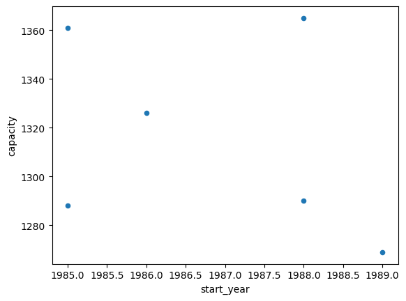
Plotting#
DataFrames have all kinds of useful plotting built in. Note that we do not even have to import matplotlib for this.
df.plot(kind="scatter", x="start_year", y="capacity")
<Axes: xlabel='start_year', ylabel='capacity'>
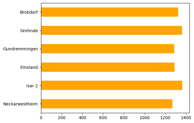
df.capacity.plot.barh(color="orange")
<Axes: >
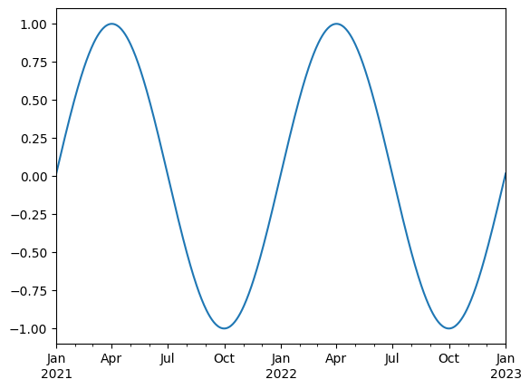
Time Indexes#
Indexes are very powerful. They are a big part of why Pandas is so useful. There are different indices for different types of data. Time Indexes are especially great when handling time-dependent data.
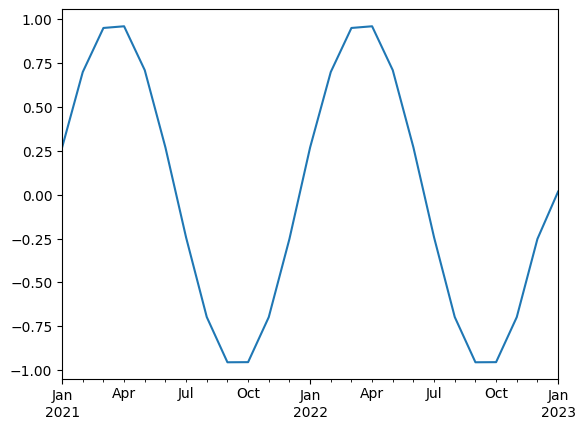
time = pd.date_range(start="2021-01-01", end="2023-01-01", freq="D")
values = np.sin(2 * np.pi * time.dayofyear / 365)
ts = pd.Series(values, index=time)
ts.plot()
<Axes: >
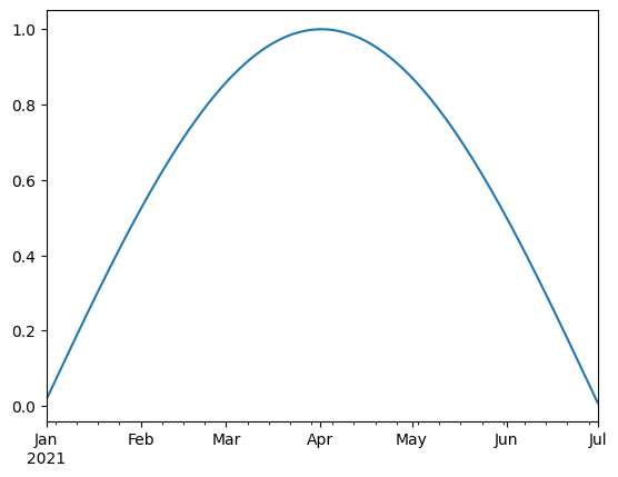
We can use Python’s slicing notation inside .loc to select a date range.
ts.loc["2021-01-01":"2021-07-01"].plot()
<Axes: >
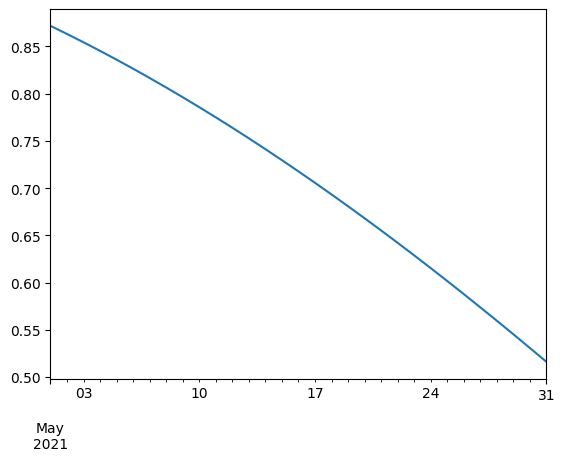
ts.loc["2021-05"].plot()
<Axes: >
The pd.TimeIndex object has lots of useful attributes
ts.index.month
Index([ 1,  1,  1,  1,  1,  1,  1,  1,  1,  1,
       ...
       12, 12, 12, 12, 12, 12, 12, 12, 12,  1],
      dtype='int32', length=731)
ts.index.day
Index([ 1,  2,  3,  4,  5,  6,  7,  8,  9, 10,
       ...
       23, 24, 25, 26, 27, 28, 29, 30, 31,  1],
      dtype='int32', length=731)
Another common operation is to change the resolution of a dataset by resampling in time. Pandas exposes this through the resample function. The resample periods are specified using pandas offset index syntax.
Below we resample the dataset by taking the mean over each month.
ts.resample("ME").mean().head()
2021-01-31    0.268746
2021-02-28    0.698782
2021-03-31    0.949778
2021-04-30    0.959332
2021-05-31    0.709200
Freq: ME, dtype: float64
ts.resample("ME").mean().plot()
<Axes: >
Reading and Writing Files#
To read data into pandas, we can use for instance the pd.read_csv() function. This function is incredibly powerful and complex with a multitude of settings. You can use it to extract data from almost any text file.
The pd.read_csv() function can take a path to a local file as an input, or even a link to an online text file.
Let’s import a slightly larger dataset about the power plant fleet in Europe_
fn = "https://raw.githubusercontent.com/PyPSA/powerplantmatching/master/powerplants.csv"
df = pd.read_csv(fn, index_col=0)
df.iloc[:5, :10]
| Name | Fueltype | Technology | Set | Country | Capacity | Efficiency | DateIn | DateRetrofit | DateOut | |
|---|---|---|---|---|---|---|---|---|---|---|
| id | ||||||||||
| 0 | Kernkraftwerk Emsland | Nuclear | Steam Turbine | PP | Germany | 1336.0 | 0.33 | 1988.0 | 1988.0 | 2023.0 |
| 1 | Brokdorf | Nuclear | Steam Turbine | PP | Germany | 1410.0 | 0.33 | 1986.0 | 1986.0 | 2021.0 |
| 2 | Borssele | Hard Coal | Steam Turbine | PP | Netherlands | 485.0 | NaN | 1973.0 | NaN | 2034.0 |
| 3 | Gemeinschaftskernkraftwerk Neckarwestheim | Nuclear | Steam Turbine | PP | Germany | 1310.0 | 0.33 | 1976.0 | 1989.0 | 2023.0 |
| 4 | Isar | Nuclear | Steam Turbine | PP | Germany | 1410.0 | 0.33 | 1979.0 | 1988.0 | 2023.0 |
df.info()
<class 'pandas.core.frame.DataFrame'>
Index: 29565 entries, 0 to 29862
Data columns (total 18 columns):
 #   Column               Non-Null Count  Dtype
---  ------               --------------  -----
 0   Name                 29565 non-null  object
 1   Fueltype             29565 non-null  object
 2   Technology           21661 non-null  object
 3   Set                  29565 non-null  object
 4   Country              29565 non-null  object
 5   Capacity             29565 non-null  float64
 6   Efficiency           541 non-null    float64
 7   DateIn               23772 non-null  float64
 8   DateRetrofit         2436 non-null   float64
 9   DateOut              932 non-null    float64
 10  lat                  29565 non-null  float64
 11  lon                  29565 non-null  float64
 12  Duration             614 non-null    float64
 13  Volume_Mm3           29565 non-null  float64
 14  DamHeight_m          29565 non-null  float64
 15  StorageCapacity_MWh  29565 non-null  float64
 16  EIC                  29565 non-null  object
 17  projectID            29565 non-null  object
dtypes: float64(11), object(7)
memory usage: 4.3+ MB
df.describe()
| Capacity | Efficiency | DateIn | DateRetrofit | DateOut | lat | lon | Duration | Volume_Mm3 | DamHeight_m | StorageCapacity_MWh | |
|---|---|---|---|---|---|---|---|---|---|---|---|
| count | 29565.000000 | 541.000000 | 23772.000000 | 2436.000000 | 932.000000 | 29565.000000 | 29565.000000 | 614.000000 | 29565.000000 | 29565.000000 | 29565.000000 |
| mean | 46.318929 | 0.480259 | 2005.777764 | 1988.509442 | 2020.609442 | 49.636627 | 9.010803 | 1290.093123 | 2.889983 | 6.463436 | 355.629403 |
| std | 198.176762 | 0.179551 | 41.415357 | 25.484325 | 10.372226 | 5.600155 | 8.090038 | 1541.197008 | 78.807802 | 46.451613 | 6634.715089 |
| min | 0.000000 | 0.140228 | 0.000000 | 1899.000000 | 1969.000000 | 32.647300 | -27.069900 | 0.007907 | 0.000000 | 0.000000 | 0.000000 |
| 25% | 2.800000 | 0.356400 | 2004.000000 | 1971.000000 | 2018.000000 | 46.861100 | 5.029700 | 90.338261 | 0.000000 | 0.000000 | 0.000000 |
| 50% | 8.200000 | 0.385600 | 2012.000000 | 1997.000000 | 2021.000000 | 50.207635 | 9.255472 | 792.753846 | 0.000000 | 0.000000 | 0.000000 |
| 75% | 25.000000 | 0.580939 | 2017.000000 | 2009.000000 | 2023.000000 | 52.630700 | 12.850190 | 2021.408119 | 0.000000 | 0.000000 | 0.000000 |
| max | 6000.000000 | 0.917460 | 2030.000000 | 2020.000000 | 2051.000000 | 71.012300 | 39.655350 | 16840.000000 | 9500.000000 | 1800.000000 | 421000.000000 |
Sometimes, we also want to store a DataFrame for later use. There are many different file formats tabular data can be stored in, including HTML, JSON, Excel, Parquet, Feather, etc. Here, let’s say we want to store the DataFrame as CSV (comma-separated values) file under the name “tmp.csv”.
df.to_csv("tmp.csv")
Groupby Functionality#
Both Series and DataFrame objects have a groupby method. It accepts a variety of arguments, but the simplest way to think about it is that you pass another series, whose unique values are used to split the original object into different groups. groupby is an amazingly powerful but also complex function.
Here’s an example which retrieves the total generation capacity per country.
grouped = df.groupby("Country").Capacity.sum()
grouped.head()
Country
Albania                    2370.400000
Austria                   24643.200368
Belgium                   21443.151009
Bosnia and Herzegovina     4827.195964
Bulgaria                  15699.186363
Name: Capacity, dtype: float64
Such “chaining” operations together is very common with pandas:
Let’s break apart this operation a bit. The workflow with groupby can be divided into three general steps:
Split: Partition the data into different groups based on some criterion.
Apply: Do some caclulation within each group. Different types of steps might be
Aggregation: Get the mean or max within the group.
Transformation: Normalize all the values within a group.
Filtration: Eliminate some groups based on a criterion.
Combine: Put the results back together into a single object.

gb = df.groupby("Country")
gb
<pandas.core.groupby.generic.DataFrameGroupBy object at 0x7fd3e79f3ed0>
The length tells us how many groups were found:
len(gb)
36
All of the groups are available as a dictionary via the .groups attribute:
groups = gb.groups
len(groups)
36
list(groups.keys())[:5]
['Albania', 'Austria', 'Belgium', 'Bosnia and Herzegovina', 'Bulgaria']
Now that we know how to create a GroupBy object, let’s learn how to do aggregation on it.
gb.Capacity.sum().nlargest(5)
Country
Germany           266203.749352
Spain             150108.858726
United Kingdom    149679.992061
France            146501.108342
Italy             101488.386461
Name: Capacity, dtype: float64
gb["DateIn"].mean().head()
Country
Albania                   1994.666667
Austria                   1987.157258
Belgium                   2001.708029
Bosnia and Herzegovina    1992.200000
Bulgaria                  1998.116279
Name: DateIn, dtype: float64
Grouping is not only possible on a single columns, but also on multiple columns. For instance,
we might want to group the capacities by country and fuel type. To achieve this, we pass a list of functions to the groupby functions.
capacities = df.groupby(["Country", "Fueltype"]).Capacity.sum()
capacities
Country         Fueltype
Albania         Hydro             1743.9
                Other               98.0
                Solar              294.5
                Wind               234.0
Austria         Hard Coal         1331.4
                                  ...
United Kingdom  Other               55.0
                Solar            11668.6
                Solid Biomass     4919.0
                Waste              288.9
                Wind             38670.3
Name: Capacity, Length: 242, dtype: float64
By grouping by multiple attributes, our index becomes a pd.MultiIndex (a hierarchical index with multiple levels.
capacities.index[:5]
MultiIndex([('Albania',     'Hydro'),
            ('Albania',     'Other'),
            ('Albania',     'Solar'),
            ('Albania',      'Wind'),
            ('Austria', 'Hard Coal')],
           names=['Country', 'Fueltype'])
type(capacities.index)
pandas.core.indexes.multi.MultiIndex
We can use the .unstack function to reshape the multi-indexed pd.Series into a pd.DataFrame which has the second index level as columns.
capacities.unstack().tail().T
| Country | Spain | Sweden | Switzerland | Ukraine | United Kingdom |
|---|---|---|---|---|---|
| Fueltype | |||||
| Biogas | NaN | NaN | NaN | NaN | 31.000000 |
| Geothermal | NaN | NaN | NaN | NaN | NaN |
| Hard Coal | 11904.878478 | 291.000000 | NaN | 24474.0 | 33823.617061 |
| Hydro | 26069.861248 | 14273.686625 | 20115.0408 | 6590.0 | 4576.175000 |
| Lignite | 1831.400000 | NaN | NaN | NaN | NaN |
| Natural Gas | 28394.244000 | 2358.000000 | 55.0000 | 4687.9 | 36366.400000 |
| Nuclear | 7733.200000 | 9859.000000 | 3355.0000 | 17635.0 | 19181.000000 |
| Oil | 1854.371000 | 1685.000000 | NaN | NaN | 100.000000 |
| Other | NaN | NaN | NaN | NaN | 55.000000 |
| Solar | 36998.200000 | 281.800000 | 96.8000 | 5628.7 | 11668.600000 |
| Solid Biomass | 563.000000 | 2432.600000 | NaN | NaN | 4919.000000 |
| Waste | 388.054000 | NaN | NaN | NaN | 288.900000 |
| Wind | 34371.650000 | 16958.800000 | 55.0000 | 461.4 | 38670.300000 |
Exercises#
Power Plants Data#
Run the function .describe() on the DataFrame that includes the power plant database:
Show code cell content
df.describe()
| Capacity | Efficiency | DateIn | DateRetrofit | DateOut | lat | lon | Duration | Volume_Mm3 | DamHeight_m | StorageCapacity_MWh | |
|---|---|---|---|---|---|---|---|---|---|---|---|
| count | 29565.000000 | 541.000000 | 23772.000000 | 2436.000000 | 932.000000 | 29565.000000 | 29565.000000 | 614.000000 | 29565.000000 | 29565.000000 | 29565.000000 |
| mean | 46.318929 | 0.480259 | 2005.777764 | 1988.509442 | 2020.609442 | 49.636627 | 9.010803 | 1290.093123 | 2.889983 | 6.463436 | 355.629403 |
| std | 198.176762 | 0.179551 | 41.415357 | 25.484325 | 10.372226 | 5.600155 | 8.090038 | 1541.197008 | 78.807802 | 46.451613 | 6634.715089 |
| min | 0.000000 | 0.140228 | 0.000000 | 1899.000000 | 1969.000000 | 32.647300 | -27.069900 | 0.007907 | 0.000000 | 0.000000 | 0.000000 |
| 25% | 2.800000 | 0.356400 | 2004.000000 | 1971.000000 | 2018.000000 | 46.861100 | 5.029700 | 90.338261 | 0.000000 | 0.000000 | 0.000000 |
| 50% | 8.200000 | 0.385600 | 2012.000000 | 1997.000000 | 2021.000000 | 50.207635 | 9.255472 | 792.753846 | 0.000000 | 0.000000 | 0.000000 |
| 75% | 25.000000 | 0.580939 | 2017.000000 | 2009.000000 | 2023.000000 | 52.630700 | 12.850190 | 2021.408119 | 0.000000 | 0.000000 | 0.000000 |
| max | 6000.000000 | 0.917460 | 2030.000000 | 2020.000000 | 2051.000000 | 71.012300 | 39.655350 | 16840.000000 | 9500.000000 | 1800.000000 | 421000.000000 |
Provide a list of unique fuel types included in the dataset
Show code cell content
df.Fueltype.unique()
array(['Nuclear', 'Hard Coal', 'Hydro', 'Lignite', 'Natural Gas', 'Oil',
       'Solid Biomass', 'Wind', 'Solar', 'Other', 'Biogas', 'Waste',
       'Geothermal'], dtype=object)
Provide a list of unique technologies included in the dataset
Show code cell content
df.Technology.unique()
array(['Steam Turbine', 'Reservoir', 'Pumped Storage', 'Run-Of-River',
       'CCGT', nan, 'Offshore', 'Onshore', 'Unknown', 'Pv', 'Marine',
       'Not Found', 'Combustion Engine', 'PV', 'CSP', 'unknown',
       'not found'], dtype=object)
Filter the dataset by power plants with the fuel type “Hard Coal”
Show code cell content
coal = df.loc[df.Fueltype == "Hard Coal"]
coal
| Name | Fueltype | Technology | Set | Country | Capacity | Efficiency | DateIn | DateRetrofit | DateOut | lat | lon | Duration | Volume_Mm3 | DamHeight_m | StorageCapacity_MWh | EIC | projectID | |
|---|---|---|---|---|---|---|---|---|---|---|---|---|---|---|---|---|---|---|
| id | ||||||||||||||||||
| 2 | Borssele | Hard Coal | Steam Turbine | PP | Netherlands | 485.000000 | NaN | 1973.0 | NaN | 2034.0 | 51.433200 | 3.716000 | NaN | 0.0 | 0.0 | 0.0 | {'49W000000000054X'} | {'BEYONDCOAL': {'BEYOND-NL-2'}, 'ENTSOE': {'49... |
| 98 | Didcot | Hard Coal | CCGT | PP | United Kingdom | 1490.000000 | 0.550000 | 1970.0 | 1998.0 | 2013.0 | 51.622300 | -1.260800 | NaN | 0.0 | 0.0 | 0.0 | {'48WSTN0000DIDCBC'} | {'BEYONDCOAL': {'BEYOND-UK-22'}, 'ENTSOE': {'4... |
| 129 | Mellach | Hard Coal | Steam Turbine | CHP | Austria | 200.000000 | NaN | 1986.0 | 1986.0 | 2020.0 | 46.911700 | 15.488300 | NaN | 0.0 | 0.0 | 0.0 | {'14W-WML-KW-----0'} | {'BEYONDCOAL': {'BEYOND-AT-11'}, 'ENTSOE': {'1... |
| 150 | Emile Huchet | Hard Coal | CCGT | PP | France | 596.493211 | NaN | 1958.0 | 2010.0 | 2022.0 | 49.152500 | 6.698100 | NaN | 0.0 | 0.0 | 0.0 | {'17W100P100P0344D', '17W100P100P0345B'} | {'BEYONDCOAL': {'BEYOND-FR-67'}, 'ENTSOE': {'1... |
| 151 | Amercoeur | Hard Coal | CCGT | PP | Belgium | 451.000000 | 0.187765 | 1968.0 | NaN | 2009.0 | 50.431000 | 4.395500 | NaN | 0.0 | 0.0 | 0.0 | {'22WAMERCO000010Y'} | {'BEYONDCOAL': {'BEYOND-BE-27'}, 'ENTSOE': {'2... |
| ... | ... | ... | ... | ... | ... | ... | ... | ... | ... | ... | ... | ... | ... | ... | ... | ... | ... | ... |
| 29779 | St | Hard Coal | NaN | CHP | Germany | 21.645000 | NaN | 1982.0 | NaN | NaN | 49.976593 | 9.068953 | NaN | 0.0 | 0.0 | 0.0 | {nan} | {'MASTR': {'MASTR-SEE971943692655'}} |
| 29804 | Uer | Hard Coal | NaN | CHP | Germany | 15.200000 | NaN | 1964.0 | NaN | NaN | 51.368132 | 6.662350 | NaN | 0.0 | 0.0 | 0.0 | {nan} | {'MASTR': {'MASTR-SEE988421065542'}} |
| 29813 | Walheim | Hard Coal | NaN | PP | Germany | 244.000000 | NaN | 1964.0 | NaN | NaN | 49.017585 | 9.157690 | NaN | 0.0 | 0.0 | 0.0 | {nan, nan} | {'MASTR': {'MASTR-SEE937157344278', 'MASTR-SEE... |
| 29830 | Wd Ffw | Hard Coal | NaN | CHP | Germany | 123.000000 | NaN | 1990.0 | NaN | NaN | 50.099000 | 8.653000 | NaN | 0.0 | 0.0 | 0.0 | {nan, nan} | {'MASTR': {'MASTR-SEE915289541482', 'MASTR-SEE... |
| 29835 | West | Hard Coal | NaN | CHP | Germany | 277.000000 | NaN | 1985.0 | NaN | NaN | 52.442456 | 10.762681 | NaN | 0.0 | 0.0 | 0.0 | {nan, nan} | {'MASTR': {'MASTR-SEE917432813484', 'MASTR-SEE... |
332 rows × 18 columns
Identify the 5 largest coal power plants. In which countries are they located? When were they built?
Show code cell content
coal.loc[coal.Capacity.nlargest(5).index]
| Name | Fueltype | Technology | Set | Country | Capacity | Efficiency | DateIn | DateRetrofit | DateOut | lat | lon | Duration | Volume_Mm3 | DamHeight_m | StorageCapacity_MWh | EIC | projectID | |
|---|---|---|---|---|---|---|---|---|---|---|---|---|---|---|---|---|---|---|
| id | ||||||||||||||||||
| 194 | Kozienice | Hard Coal | Steam Turbine | PP | Poland | 3682.216205 | NaN | 1972.0 | NaN | 2042.0 | 51.6647 | 21.4667 | NaN | 0.0 | 0.0 | 0.0 | {'19W000000000104I', '19W000000000095U'} | {'BEYONDCOAL': {'BEYOND-PL-96'}, 'ENTSOE': {'1... |
| 3652 | Vuglegirska | Hard Coal | CCGT | PP | Ukraine | 3600.000000 | NaN | 1972.0 | NaN | NaN | 48.4652 | 38.2027 | NaN | 0.0 | 0.0 | 0.0 | {nan} | {'GPD': {'WRI1005107'}, 'GEO': {'GEO-43001'}} |
| 767 | Opole | Hard Coal | Steam Turbine | PP | Poland | 3071.893939 | NaN | 1993.0 | NaN | 2020.0 | 50.7518 | 17.8820 | NaN | 0.0 | 0.0 | 0.0 | {'19W0000000001292'} | {'BEYONDCOAL': {'BEYOND-PL-16'}, 'ENTSOE': {'1... |
| 3651 | Zaporizhia | Hard Coal | CCGT | PP | Ukraine | 2825.000000 | NaN | 1972.0 | NaN | NaN | 47.5089 | 34.6253 | NaN | 0.0 | 0.0 | 0.0 | {nan} | {'GPD': {'WRI1005101'}, 'GEO': {'GEO-42988'}} |
| 3704 | Moldavskaya Gres | Hard Coal | CCGT | PP | Moldova | 2520.000000 | NaN | 1964.0 | NaN | NaN | 46.6292 | 29.9407 | NaN | 0.0 | 0.0 | 0.0 | {nan} | {'GPD': {'WRI1002989'}, 'GEO': {'GEO-43028'}} |
Identify the power plant with the longest “Name”.
Show code cell content
i = df.Name.map(lambda x: len(x)).argmax()
df.iloc[i]
Name                   Kesznyeten Hernadviz Hungary Kesznyeten Hernad...
Fueltype                                                           Hydro
Technology                                                  Run-Of-River
Set                                                                   PP
Country                                                          Hungary
Capacity                                                             4.4
Efficiency                                                           NaN
DateIn                                                            1945.0
DateRetrofit                                                      1992.0
DateOut                                                              NaN
lat                                                            47.995972
lon                                                            21.033037
Duration                                                             NaN
Volume_Mm3                                                           0.0
DamHeight_m                                                         14.0
StorageCapacity_MWh                                                  0.0
EIC                                                                {nan}
projectID                   {'JRC': {'JRC-H2138'}, 'GEO': {'GEO-42677'}}
Name: 2595, dtype: object
Identify the 10 northernmost powerplants. What type of power plants are they?
Show code cell content
index = df.lat.nlargest(10).index
df.loc[index]
| Name | Fueltype | Technology | Set | Country | Capacity | Efficiency | DateIn | DateRetrofit | DateOut | lat | lon | Duration | Volume_Mm3 | DamHeight_m | StorageCapacity_MWh | EIC | projectID | |
|---|---|---|---|---|---|---|---|---|---|---|---|---|---|---|---|---|---|---|
| id | ||||||||||||||||||
| 13729 | Havoygavlen Wind Farm | Wind | Onshore | PP | Norway | 78.0 | NaN | 2003.0 | NaN | 2021.0 | 71.012300 | 24.594200 | NaN | 0.0 | 0.0 | 0.0 | {nan, nan} | {'GEM': {'G100000917445', 'G100000917626'}} |
| 14629 | Kjollefjord Wind Farm | Wind | Onshore | PP | Norway | 39.0 | NaN | 2006.0 | NaN | NaN | 70.918500 | 27.289900 | NaN | 0.0 | 0.0 | 0.0 | {nan} | {'GEM': {'G100000917523'}} |
| 4385 | Repvag | Hydro | Reservoir | Store | Norway | 4.4 | NaN | 1953.0 | 1953.0 | NaN | 70.773547 | 25.616486 | 2810.704545 | 28.3 | 172.0 | 12367.1 | {nan} | {'JRC': {'JRC-N339'}, 'OPSD': {'OEU-4174'}} |
| 18578 | Raggovidda Wind Farm | Wind | Onshore | PP | Norway | 97.0 | NaN | 2014.0 | NaN | NaN | 70.765700 | 29.083300 | NaN | 0.0 | 0.0 | 0.0 | {nan, nan} | {'GEM': {'G100000918729', 'G100000918029'}} |
| 5363 | Maroyfjord | Hydro | Reservoir | Store | Norway | 4.4 | NaN | 1956.0 | 1956.0 | NaN | 70.751421 | 27.355047 | 1533.681818 | 13.8 | 225.3 | 6748.2 | {nan} | {'JRC': {'JRC-N289'}, 'OPSD': {'OEU-4036'}} |
| 6506 | Melkoya | Natural Gas | CCGT | PP | Norway | 230.0 | NaN | 2007.0 | 2007.0 | NaN | 70.689366 | 23.600448 | NaN | 0.0 | 0.0 | 0.0 | {'50WP00000000456T'} | {'ENTSOE': {'50WP00000000456T'}, 'OPSD': {'OEU... |
| 13634 | Hammerfest Snohvit Terminal | Natural Gas | CCGT | PP | Norway | 229.0 | NaN | NaN | NaN | NaN | 70.685400 | 23.590000 | NaN | 0.0 | 0.0 | 0.0 | {nan} | {'GEM': {'L100000407847'}} |
| 13636 | Hamnefjell Wind Farm | Wind | Onshore | PP | Norway | 52.0 | NaN | 2017.0 | NaN | NaN | 70.667900 | 29.719000 | NaN | 0.0 | 0.0 | 0.0 | {nan} | {'GEM': {'G100000918725'}} |
| 5425 | Hammerfest | Hydro | Reservoir | Store | Norway | 1.1 | NaN | 1947.0 | 1947.0 | NaN | 70.657936 | 23.714418 | 1638.181818 | 10.6 | 88.0 | 1802.0 | {nan} | {'JRC': {'JRC-N127'}, 'OPSD': {'OEU-3550'}} |
| 5270 | Kongsfjord | Hydro | Reservoir | Store | Norway | 4.4 | NaN | 1946.0 | 1946.0 | NaN | 70.598729 | 29.057905 | 3343.795455 | 88.1 | 70.5 | 14712.7 | {nan} | {'JRC': {'JRC-N210'}, 'OPSD': {'OEU-3801'}} |
What is the average “DateIn” of each “Fueltype”? Which type of power plants is the oldest on average?
Show code cell content
df.groupby("Fueltype").DateIn.mean().sort_values()
Fueltype
Hard Coal        1971.907407
Hydro            1972.767529
Nuclear          1975.785047
Lignite          1976.815789
Other            1992.456897
Waste            1997.154412
Geothermal       2000.142857
Oil              2000.589862
Solid Biomass    2001.483412
Natural Gas      2001.918495
Wind             2009.516211
Biogas           2012.584270
Solar            2015.415509
Name: DateIn, dtype: float64
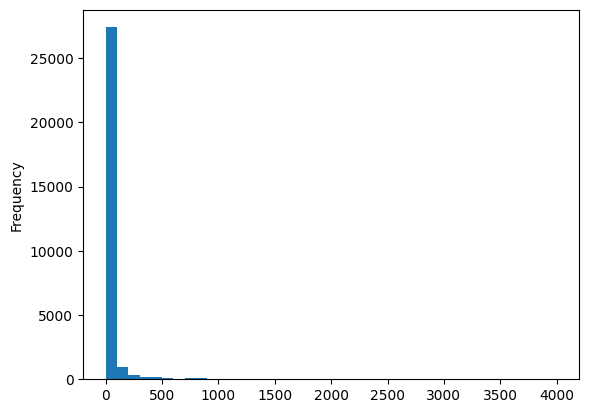
Plot a histogram of power plant capacities with bins of length 100 MW between 0 and 4000 MW. What do you observe?
Show code cell content
df.Capacity.plot.hist(bins=np.arange(0, 4001, 100))
<Axes: ylabel='Frequency'>
How many power plants of each fuel type are there in each country? Display the results in a DataFrame with countries as index and fuel type as columns. Fill missing values with the value zero. Convert all values to integers.
Browse Google or the pandas documentation to find the right aggregation function to count values.
Show code cell content
df.groupby(["Country", "Fueltype"]).size().unstack().fillna(0.0).astype(int)
| Fueltype | Biogas | Geothermal | Hard Coal | Hydro | Lignite | Natural Gas | Nuclear | Oil | Other | Solar | Solid Biomass | Waste | Wind |
|---|---|---|---|---|---|---|---|---|---|---|---|---|---|
| Country | |||||||||||||
| Albania | 0 | 0 | 0 | 10 | 0 | 0 | 0 | 0 | 1 | 11 | 0 | 0 | 1 |
| Austria | 0 | 0 | 6 | 175 | 2 | 19 | 0 | 0 | 0 | 61 | 0 | 0 | 93 |
| Belgium | 0 | 0 | 10 | 13 | 0 | 27 | 3 | 8 | 0 | 76 | 6 | 8 | 89 |
| Bosnia and Herzegovina | 0 | 0 | 0 | 17 | 10 | 0 | 0 | 0 | 0 | 19 | 0 | 0 | 7 |
| Bulgaria | 0 | 0 | 4 | 30 | 9 | 6 | 1 | 0 | 0 | 215 | 0 | 0 | 17 |
| Croatia | 0 | 0 | 1 | 21 | 0 | 7 | 0 | 0 | 0 | 26 | 0 | 0 | 27 |
| Czechia | 0 | 0 | 11 | 14 | 27 | 8 | 2 | 0 | 0 | 331 | 1 | 0 | 6 |
| Denmark | 0 | 0 | 12 | 0 | 0 | 13 | 0 | 1 | 1 | 73 | 9 | 0 | 112 |
| Estonia | 0 | 0 | 0 | 0 | 0 | 2 | 0 | 2 | 0 | 71 | 0 | 0 | 15 |
| Finland | 25 | 0 | 17 | 105 | 6 | 32 | 2 | 12 | 3 | 13 | 21 | 0 | 155 |
| France | 0 | 0 | 16 | 155 | 1 | 42 | 23 | 6 | 2 | 1268 | 5 | 0 | 1054 |
| Germany | 531 | 0 | 87 | 972 | 46 | 992 | 26 | 404 | 109 | 5010 | 67 | 119 | 5180 |
| Greece | 0 | 0 | 0 | 20 | 10 | 18 | 0 | 0 | 0 | 315 | 0 | 1 | 192 |
| Hungary | 0 | 0 | 5 | 4 | 1 | 17 | 1 | 1 | 0 | 319 | 4 | 0 | 10 |
| Ireland | 0 | 0 | 1 | 6 | 2 | 17 | 0 | 4 | 0 | 33 | 1 | 0 | 123 |
| Italy | 0 | 25 | 18 | 289 | 0 | 122 | 4 | 2 | 2 | 249 | 12 | 0 | 280 |
| Kosovo | 0 | 0 | 0 | 2 | 2 | 0 | 0 | 0 | 0 | 4 | 0 | 0 | 2 |
| Latvia | 0 | 0 | 0 | 3 | 0 | 3 | 0 | 0 | 0 | 12 | 0 | 0 | 3 |
| Lithuania | 0 | 0 | 0 | 2 | 0 | 4 | 1 | 0 | 0 | 32 | 1 | 0 | 23 |
| Luxembourg | 0 | 0 | 0 | 1 | 0 | 0 | 0 | 0 | 0 | 16 | 0 | 0 | 9 |
| Moldova | 0 | 0 | 1 | 1 | 0 | 2 | 0 | 0 | 0 | 8 | 0 | 0 | 0 |
| Montenegro | 0 | 0 | 0 | 4 | 1 | 0 | 0 | 0 | 0 | 1 | 0 | 0 | 2 |
| Netherlands | 1 | 0 | 9 | 0 | 0 | 54 | 1 | 0 | 2 | 221 | 12 | 0 | 148 |
| North Macedonia | 0 | 0 | 0 | 10 | 2 | 2 | 0 | 0 | 0 | 34 | 0 | 0 | 2 |
| Norway | 0 | 0 | 0 | 930 | 0 | 4 | 0 | 0 | 0 | 1 | 0 | 0 | 60 |
| Poland | 0 | 0 | 54 | 19 | 8 | 22 | 0 | 1 | 0 | 291 | 6 | 0 | 223 |
| Portugal | 0 | 0 | 3 | 44 | 0 | 18 | 0 | 0 | 0 | 92 | 4 | 0 | 125 |
| Romania | 0 | 0 | 3 | 119 | 15 | 15 | 1 | 0 | 0 | 231 | 1 | 0 | 48 |
| Serbia | 0 | 0 | 0 | 13 | 10 | 3 | 0 | 0 | 0 | 9 | 1 | 0 | 10 |
| Slovakia | 0 | 0 | 4 | 29 | 3 | 6 | 2 | 0 | 0 | 105 | 0 | 0 | 0 |
| Slovenia | 0 | 0 | 1 | 28 | 4 | 3 | 1 | 0 | 0 | 7 | 0 | 0 | 0 |
| Spain | 0 | 0 | 22 | 359 | 7 | 88 | 7 | 12 | 0 | 1288 | 11 | 15 | 843 |
| Sweden | 0 | 0 | 2 | 147 | 0 | 12 | 5 | 4 | 0 | 37 | 35 | 0 | 254 |
| Switzerland | 0 | 0 | 0 | 472 | 0 | 1 | 5 | 0 | 0 | 48 | 0 | 0 | 3 |
| Ukraine | 0 | 0 | 19 | 9 | 0 | 11 | 5 | 0 | 0 | 427 | 0 | 0 | 11 |
| United Kingdom | 2 | 0 | 26 | 101 | 0 | 93 | 17 | 1 | 1 | 1137 | 36 | 10 | 406 |
Time Series Analysis#
Read in the time series from the second lecture into a DataFrame.
The file is available at https://tubcloud.tu-berlin.de/s/pKttFadrbTKSJKF/download/time-series-lecture-2.csv. and includes hourly time series for Germany in 2015 for:
electricity demand from OPSD in GW
onshore wind capacity factors from renewables.ninja in per-unit of installed capacity
offshore wind capacity factors from renewables.ninja in per-unit of installed capacity
solar PV capacity factors from renewables.ninja in per-unit of installed capacity
electricity day-ahead spot market prices in €/MWh from EPEX Spot zone DE/AT/LU retrieved via SMARD platform
Use the function pd.read_csv with the keyword arguments index_col= and parse_dates= to ensure the
time stamps are treated as pd.DatetimeIndex.
# your code here
The start of the DataFrame should look like this:
load |
onwind |
offwind |
solar |
prices |
|
|---|---|---|---|---|---|
2015-01-01 00:00:00 |
41.151 |
0.1566 |
0.703 |
0 |
nan |
2015-01-01 01:00:00 |
40.135 |
0.1659 |
0.6875 |
0 |
nan |
2015-01-01 02:00:00 |
39.106 |
0.1746 |
0.6535 |
0 |
nan |
2015-01-01 03:00:00 |
38.765 |
0.1745 |
0.6803 |
0 |
nan |
2015-01-01 04:00:00 |
38.941 |
0.1826 |
0.7272 |
0 |
nan |
And it should pass the following test:
assert type(df.index) == pd.DatetimeIndex
For each column:
What are the average, minimum and maximum values?
Find the time stamps where data on prices is missing.
Fill up the missing data with the prices observed one week ahead.
Plot the time series for the full year.
Plot the time series for the month May.
Resample the time series to daily, weeky, and monthly frequencies and plot the resulting time series in one graph.
Sort the values in descending order and plot the duration curve. Hint: Run
.reset_index(drop=True)to drop the index after sorting.Plot a histogram of the time series values.
Perform a Fourier transformation of the time series. What are the dominant frequencies? Hint: Below you can find an example how Fourier transformation can be down with
numpy.Calculate the Pearson correlation coefficients between all time series. Hint: There is a function for that. Google for “pandas dataframe correlation”.
abs(pd.Series(np.fft.rfft(df.solar - df.solar.mean()), index=np.fft.rfftfreq(len(df.solar), d=1./8760))**2)
# your code here