Preparation for Group Assignment

This tutorial contains various small guides for tasks you will need or come in handy in the upcoming group assignment.

We’re going to need a couple of packages for this tutorial:

from atlite.gis import ExclusionContainer
from atlite.gis import shape_availability
import atlite
from rasterio.plot import show
import geopandas as gpd
import pandas as pd
import xarray as xr
import matplotlib.pyplot as plt
import country_converter as coco
import atlite

Preparatory Downloads

For this tutorial, we also need to download a few files, for which one can use the urllib library:

Show code cell content Hide code cell content

from urllib.request import urlretrieve

Show code cell content Hide code cell content

fn = "era5-2013-NL.nc"
url = "https://tubcloud.tu-berlin.de/s/bAJj9xmN5ZLZQZJ/download/" + fn
urlretrieve(url, fn)

('era5-2013-NL.nc', <http.client.HTTPMessage at 0x7f5a202de050>)

Show code cell content Hide code cell content

fn = "PROBAV_LC100_global_v3.0.1_2019-nrt_Discrete-Classification-map_EPSG-4326-NL.tif"
url = f"https://tubcloud.tu-berlin.de/s/567ckizz2Y6RLQq/download?path=%2Fcopernicus-glc&files={fn}"
urlretrieve(url, fn)

('PROBAV_LC100_global_v3.0.1_2019-nrt_Discrete-Classification-map_EPSG-4326-NL.tif',
 <http.client.HTTPMessage at 0x7f5a2035a590>)

Show code cell content Hide code cell content

fn = "WDPA_Oct2022_Public_shp-NLD.tif"
url = (
    f"https://tubcloud.tu-berlin.de/s/567ckizz2Y6RLQq/download?path=%2Fwdpa&files={fn}"
)
urlretrieve(url, fn)

('WDPA_Oct2022_Public_shp-NLD.tif',
 <http.client.HTTPMessage at 0x7f5a20360310>)

Show code cell content Hide code cell content

fn = "GEBCO_2014_2D-NL.nc"
url = (
    f"https://tubcloud.tu-berlin.de/s/567ckizz2Y6RLQq/download?path=%2Fgebco&files={fn}"
)
urlretrieve(url, fn)

('GEBCO_2014_2D-NL.nc', <http.client.HTTPMessage at 0x7f5a20362190>)

Downloading historical weather data from ERA5 with atlite

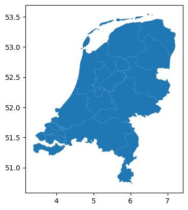
First, let’s load some small example country. Let’s say, the Netherlands.

fn = "https://tubcloud.tu-berlin.de/s/567ckizz2Y6RLQq/download?path=%2Fgadm&files=gadm_410-levels-ADM_1-NLD.gpkg"
regions = gpd.read_file(fn)

/opt/hostedtoolcache/Python/3.11.11/x64/lib/python3.11/site-packages/pyogrio/raw.py:198: RuntimeWarning: File /vsimem/pyogrio_fc70a2516b214ae9b393a12b795dfe34 has GPKG application_id, but non conformant file extension
  return ogr_read(

regions.plot()

<Axes: >

In this example we download historical weather data ERA5 data on-demand for a cutout we want to create.

Note

For this example to work, you should have

• installed the Copernicus Climate Data Store cdsapi package (conda list cdsapi or pip install cdsapi) and

• registered and setup your CDS API key as described on this website. Note that there are different instructions depending on your operating system.

A cutout is the basis for any of your work and calculations in atlite.

The cutout is created in the directory and file specified by the relative path. If a cutout at the given location already exists, then this command will simply load the cutout again. If the cutout does not yet exist, it will specify the new cutout to be created.

For creating the cutout, you need to specify the dataset (e.g. ERA5), a time period and the spatial extent (in latitude and longitude).

minx, miny, maxx, maxy = regions.total_bounds
buffer = 0.25

cutout = atlite.Cutout(
    path="era5-2013-NL.nc",
    module="era5",
    x=slice(minx - buffer, maxx + buffer),
    y=slice(miny - buffer, maxy + buffer),
    time="2013",
)

/opt/hostedtoolcache/Python/3.11.11/x64/lib/python3.11/site-packages/atlite/cutout.py:156: UserWarning: Arguments module, x, y, time are ignored, since cutout is already built.
  warn(

Calling the function cutout.prepare() initiates the download and processing of the weather data. Because the download needs to be provided by the CDS servers, this might take a while depending on the amount of data requested.

Note

You can check the status of your request here.

# cutout.prepare(compression=None)

The data is accessible in cutout.data. Included weather variables are listed in cutout.prepared_features. Querying the cutout gives us some basic information on which data is contained in it.

cutout.data

<xarray.Dataset> Size: 134MB
Dimensions:           (x: 17, y: 14, time: 8760)
Coordinates:
  * x                 (x) float64 136B 3.25 3.5 3.75 4.0 ... 6.5 6.75 7.0 7.25
  * y                 (y) float64 112B 50.5 50.75 51.0 ... 53.25 53.5 53.75
  * time              (time) datetime64[ns] 70kB 2013-01-01 ... 2013-12-31T23...
    lon               (x) float64 136B dask.array<chunksize=(17,), meta=np.ndarray>
    lat               (y) float64 112B dask.array<chunksize=(14,), meta=np.ndarray>
Data variables: (12/13)
    height            (y, x) float32 952B dask.array<chunksize=(14, 17), meta=np.ndarray>
    wnd100m           (time, y, x) float32 8MB dask.array<chunksize=(100, 14, 17), meta=np.ndarray>
    wnd_azimuth       (time, y, x) float32 8MB dask.array<chunksize=(100, 14, 17), meta=np.ndarray>
    roughness         (time, y, x) float32 8MB dask.array<chunksize=(100, 14, 17), meta=np.ndarray>
    influx_toa        (time, y, x) float32 8MB dask.array<chunksize=(100, 14, 17), meta=np.ndarray>
    influx_direct     (time, y, x) float32 8MB dask.array<chunksize=(100, 14, 17), meta=np.ndarray>
    ...                ...
    albedo            (time, y, x) float32 8MB dask.array<chunksize=(100, 14, 17), meta=np.ndarray>
    solar_altitude    (time, y, x) float64 17MB dask.array<chunksize=(100, 14, 17), meta=np.ndarray>
    solar_azimuth     (time, y, x) float64 17MB dask.array<chunksize=(100, 14, 17), meta=np.ndarray>
    temperature       (time, y, x) float64 17MB dask.array<chunksize=(100, 14, 17), meta=np.ndarray>
    soil temperature  (time, y, x) float64 17MB dask.array<chunksize=(100, 14, 17), meta=np.ndarray>
    runoff            (time, y, x) float32 8MB dask.array<chunksize=(100, 14, 17), meta=np.ndarray>
Attributes:
    module:             era5
    prepared_features:  ['influx', 'wind', 'height', 'temperature', 'runoff']
    chunksize_time:     100
    Conventions:        CF-1.6
    history:            2023-01-15 21:33:09 GMT by grib_to_netcdf-2.25.1: /op...

xarray.Dataset

• Dimensions:
  • x: 17
  • y: 14
  • time: 8760
• Coordinates: (5)
  • x
    (x)
    float64
    3.25 3.5 3.75 4.0 ... 6.75 7.0 7.25

    array([3.25, 3.5 , 3.75, 4.  , 4.25, 4.5 , 4.75, 5.  , 5.25, 5.5 , 5.75, 6.  ,
           6.25, 6.5 , 6.75, 7.  , 7.25])

  • y
    (y)
    float64
    50.5 50.75 51.0 ... 53.5 53.75

    array([50.5 , 50.75, 51.  , 51.25, 51.5 , 51.75, 52.  , 52.25, 52.5 , 52.75,
           53.  , 53.25, 53.5 , 53.75])

  • time
    (time)
    datetime64[ns]
    2013-01-01 ... 2013-12-31T23:00:00

    array(['2013-01-01T00:00:00.000000000', '2013-01-01T01:00:00.000000000',
           '2013-01-01T02:00:00.000000000', ..., '2013-12-31T21:00:00.000000000',
           '2013-12-31T22:00:00.000000000', '2013-12-31T23:00:00.000000000'],
          dtype='datetime64[ns]')

  • lon
    (x)
    float64
    dask.array<chunksize=(17,), meta=np.ndarray>

    Array Chunk Bytes 136 B 136 B Shape (17,) (17,) Dask graph 1 chunks in 2 graph layers Data type float64 numpy.ndarray

  • lat
    (y)
    float64
    dask.array<chunksize=(14,), meta=np.ndarray>

    Array Chunk Bytes 112 B 112 B Shape (14,) (14,) Dask graph 1 chunks in 2 graph layers Data type float64 numpy.ndarray

• Data variables: (13)
  • height
    (y, x)
    float32
    dask.array<chunksize=(14, 17), meta=np.ndarray>

    module :

    era5

    feature :

    height

    Array Chunk Bytes 0.93 kiB 0.93 kiB Shape (14, 17) (14, 17) Dask graph 1 chunks in 2 graph layers Data type float32 numpy.ndarray

  • wnd100m
    (time, y, x)
    float32
    dask.array<chunksize=(100, 14, 17), meta=np.ndarray>

    units :

    m s**-1

    long_name :

    100 metre wind speed

    module :

    era5

    feature :

    wind

    Array Chunk Bytes 7.95 MiB 92.97 kiB Shape (8760, 14, 17) (100, 14, 17) Dask graph 88 chunks in 2 graph layers Data type float32 numpy.ndarray

  • wnd_azimuth
    (time, y, x)
    float32
    dask.array<chunksize=(100, 14, 17), meta=np.ndarray>

    units :

    m s**-1

    long_name :

    100 metre U wind component

    module :

    era5

    feature :

    wind

    Array Chunk Bytes 7.95 MiB 92.97 kiB Shape (8760, 14, 17) (100, 14, 17) Dask graph 88 chunks in 2 graph layers Data type float32 numpy.ndarray

  • roughness
    (time, y, x)
    float32
    dask.array<chunksize=(100, 14, 17), meta=np.ndarray>

    units :

    m

    long_name :

    Forecast surface roughness

    module :

    era5

    feature :

    wind

    Array Chunk Bytes 7.95 MiB 92.97 kiB Shape (8760, 14, 17) (100, 14, 17) Dask graph 88 chunks in 2 graph layers Data type float32 numpy.ndarray

  • influx_toa
    (time, y, x)
    float32
    dask.array<chunksize=(100, 14, 17), meta=np.ndarray>

    units :

    W m**-2

    module :

    era5

    feature :

    influx

    Array Chunk Bytes 7.95 MiB 92.97 kiB Shape (8760, 14, 17) (100, 14, 17) Dask graph 88 chunks in 2 graph layers Data type float32 numpy.ndarray

  • influx_direct
    (time, y, x)
    float32
    dask.array<chunksize=(100, 14, 17), meta=np.ndarray>

    units :

    W m**-2

    module :

    era5

    feature :

    influx

    Array Chunk Bytes 7.95 MiB 92.97 kiB Shape (8760, 14, 17) (100, 14, 17) Dask graph 88 chunks in 2 graph layers Data type float32 numpy.ndarray

  • influx_diffuse
    (time, y, x)
    float32
    dask.array<chunksize=(100, 14, 17), meta=np.ndarray>

    units :

    W m**-2

    module :

    era5

    feature :

    influx

    Array Chunk Bytes 7.95 MiB 92.97 kiB Shape (8760, 14, 17) (100, 14, 17) Dask graph 88 chunks in 2 graph layers Data type float32 numpy.ndarray

  • albedo
    (time, y, x)
    float32
    dask.array<chunksize=(100, 14, 17), meta=np.ndarray>

    units :

    (0 - 1)

    long_name :

    Albedo

    module :

    era5

    feature :

    influx

    Array Chunk Bytes 7.95 MiB 92.97 kiB Shape (8760, 14, 17) (100, 14, 17) Dask graph 88 chunks in 2 graph layers Data type float32 numpy.ndarray

  • solar_altitude
    (time, y, x)
    float64
    dask.array<chunksize=(100, 14, 17), meta=np.ndarray>

    time shift :

    -1 days +23:30:00

    units :

    rad

    module :

    era5

    feature :

    influx

    Array Chunk Bytes 15.91 MiB 185.94 kiB Shape (8760, 14, 17) (100, 14, 17) Dask graph 88 chunks in 2 graph layers Data type float64 numpy.ndarray

  • solar_azimuth
    (time, y, x)
    float64
    dask.array<chunksize=(100, 14, 17), meta=np.ndarray>

    time shift :

    -1 days +23:30:00

    units :

    rad

    module :

    era5

    feature :

    influx

    Array Chunk Bytes 15.91 MiB 185.94 kiB Shape (8760, 14, 17) (100, 14, 17) Dask graph 88 chunks in 2 graph layers Data type float64 numpy.ndarray

  • temperature
    (time, y, x)
    float64
    dask.array<chunksize=(100, 14, 17), meta=np.ndarray>

    units :

    K

    long_name :

    2 metre temperature

    module :

    era5

    feature :

    temperature

    Array Chunk Bytes 15.91 MiB 185.94 kiB Shape (8760, 14, 17) (100, 14, 17) Dask graph 88 chunks in 2 graph layers Data type float64 numpy.ndarray

  • soil temperature
    (time, y, x)
    float64
    dask.array<chunksize=(100, 14, 17), meta=np.ndarray>

    units :

    K

    long_name :

    Soil temperature level 4

    module :

    era5

    feature :

    temperature

    Array Chunk Bytes 15.91 MiB 185.94 kiB Shape (8760, 14, 17) (100, 14, 17) Dask graph 88 chunks in 2 graph layers Data type float64 numpy.ndarray

  • runoff
    (time, y, x)
    float32
    dask.array<chunksize=(100, 14, 17), meta=np.ndarray>

    units :

    m

    long_name :

    Runoff

    module :

    era5

    feature :

    runoff

    Array Chunk Bytes 7.95 MiB 92.97 kiB Shape (8760, 14, 17) (100, 14, 17) Dask graph 88 chunks in 2 graph layers Data type float32 numpy.ndarray

• Indexes: (3)
  • x
    PandasIndex

    PandasIndex(Index([3.25,  3.5, 3.75,  4.0, 4.25,  4.5, 4.75,  5.0, 5.25,  5.5, 5.75,  6.0,
           6.25,  6.5, 6.75,  7.0, 7.25],
          dtype='float64', name='x'))

  • y
    PandasIndex

    PandasIndex(Index([ 50.5, 50.75,  51.0, 51.25,  51.5, 51.75,  52.0, 52.25,  52.5, 52.75,
            53.0, 53.25,  53.5, 53.75],
          dtype='float64', name='y'))

  • time
    PandasIndex

    PandasIndex(DatetimeIndex(['2013-01-01 00:00:00', '2013-01-01 01:00:00',
                   '2013-01-01 02:00:00', '2013-01-01 03:00:00',
                   '2013-01-01 04:00:00', '2013-01-01 05:00:00',
                   '2013-01-01 06:00:00', '2013-01-01 07:00:00',
                   '2013-01-01 08:00:00', '2013-01-01 09:00:00',
                   ...
                   '2013-12-31 14:00:00', '2013-12-31 15:00:00',
                   '2013-12-31 16:00:00', '2013-12-31 17:00:00',
                   '2013-12-31 18:00:00', '2013-12-31 19:00:00',
                   '2013-12-31 20:00:00', '2013-12-31 21:00:00',
                   '2013-12-31 22:00:00', '2013-12-31 23:00:00'],
                  dtype='datetime64[ns]', name='time', length=8760, freq=None))

• Attributes: (5)

  module :

  era5

  prepared_features :

  ['influx', 'wind', 'height', 'temperature', 'runoff']

  chunksize_time :

  100

  Conventions :

  CF-1.6

  history :

  2023-01-15 21:33:09 GMT by grib_to_netcdf-2.25.1: /opt/ecmwf/mars-client/bin/grib_to_netcdf.bin -S param -o /cache/data3/adaptor.mars.internal-1673818389.308055-17097-17-6421fb9f-1d14-49f0-9bc9-95159f10ea37.nc /cache/tmp/6421fb9f-1d14-49f0-9bc9-95159f10ea37-adaptor.mars.internal-1673818388.7901623-17097-20-tmp.grib

cutout.prepared_features

module  feature    
era5    height                   height
        wind                    wnd100m
        wind                wnd_azimuth
        wind                  roughness
        influx               influx_toa
        influx            influx_direct
        influx           influx_diffuse
        influx                   albedo
        influx           solar_altitude
        influx            solar_azimuth
        temperature         temperature
        temperature    soil temperature
        runoff                   runoff
dtype: object

cutout

<Cutout "era5-2013-NL">
 x = 3.25 ⟷ 7.25, dx = 0.25
 y = 50.50 ⟷ 53.75, dy = 0.25
 time = 2013-01-01 ⟷ 2013-12-31, dt = h
 module = era5
 prepared_features = ['height', 'wind', 'influx', 'temperature', 'runoff']

Repetition: From Land Eligibility Analysis to Availability Matrix

We’re going to use the plotting functions from previous exercises:

def plot_area(masked, transform, shape):
    fig, ax = plt.subplots(figsize=(5, 5))
    ax = show(masked, transform=transform, cmap="Greens", vmin=0, ax=ax)
    shape.plot(ax=ax, edgecolor="k", color="None", linewidth=1)

First, we collect all exclusion and inclusion criteria in an ExclusionContainer.

excluder = ExclusionContainer(crs=3035, res=300)
fn = "PROBAV_LC100_global_v3.0.1_2019-nrt_Discrete-Classification-map_EPSG-4326-NL.tif"
excluder.add_raster(fn, codes=[50], buffer=1000, crs=4326)
excluder.add_raster(fn, codes=[20, 30, 40, 60], crs=4326, invert=True)
fn = "WDPA_Oct2022_Public_shp-NLD.tif"
excluder.add_raster(fn, crs=3035)
fn = "GEBCO_2014_2D-NL.nc"
excluder.add_raster(fn, codes=lambda x: x > 10, crs=4326, invert=True)

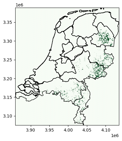
Then, we can calculate the available areas…

masked, transform = shape_availability(regions.to_crs(3035).geometry, excluder)

… and plot it:

plot_area(masked, transform, regions.to_crs(3035).geometry)

Availability Matrix

regions.index = regions.GID_1

cutout = atlite.Cutout("era5-2013-NL.nc")

?cutout.availabilitymatrix

A = cutout.availabilitymatrix(regions, excluder)

cap_per_sqkm = 1.7  # MW/km2

area = cutout.grid.set_index(["y", "x"]).to_crs(3035).area / 1e6

area = xr.DataArray(area, dims=("spatial"))

capacity_matrix = A.stack(spatial=["y", "x"]) * area * cap_per_sqkm

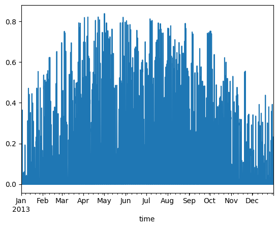
Solar PV Profiles

pv = cutout.pv(
    panel=atlite.solarpanels.CdTe,
    matrix=capacity_matrix,
    orientation="latitude_optimal",
    index=regions.index,
    per_unit=True,
)

pv.to_pandas().head()

GID_1	NLD.1_1	NLD.2_1	NLD.3_1	NLD.4_1	NLD.5_1	NLD.6_1	NLD.7_1	NLD.8_1	NLD.9_1	NLD.10_1	NLD.11_1	NLD.12_1	NLD.13_1	NLD.14_1
time
2013-01-01 00:00:00	0.0	0.0	0.0	0.0	0.0	0.0	0.0	0.0	0.0	0.0	0.0	0.0	0.0	0.0
2013-01-01 01:00:00	0.0	0.0	0.0	0.0	0.0	0.0	0.0	0.0	0.0	0.0	0.0	0.0	0.0	0.0
2013-01-01 02:00:00	0.0	0.0	0.0	0.0	0.0	0.0	0.0	0.0	0.0	0.0	0.0	0.0	0.0	0.0
2013-01-01 03:00:00	0.0	0.0	0.0	0.0	0.0	0.0	0.0	0.0	0.0	0.0	0.0	0.0	0.0	0.0
2013-01-01 04:00:00	0.0	0.0	0.0	0.0	0.0	0.0	0.0	0.0	0.0	0.0	0.0	0.0	0.0	0.0

pv.to_pandas().iloc[:, 0].plot()

<Axes: xlabel='time'>

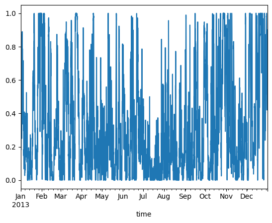
Wind Profiles

wind = cutout.wind(
    atlite.windturbines.Vestas_V112_3MW,
    matrix=capacity_matrix,
    index=regions.index,
    per_unit=True,
)

/opt/hostedtoolcache/Python/3.11.11/x64/lib/python3.11/site-packages/atlite/resource.py:90: FutureWarning: 'add_cutout_windspeed' for wind turbine
power curves will default to True in atlite relase v0.2.15.
  warnings.warn(msg, FutureWarning)

wind.to_pandas().head()

GID_1	NLD.1_1	NLD.2_1	NLD.3_1	NLD.4_1	NLD.5_1	NLD.6_1	NLD.7_1	NLD.8_1	NLD.9_1	NLD.10_1	NLD.11_1	NLD.12_1	NLD.13_1	NLD.14_1
time
2013-01-01 00:00:00	0.999056	0.998485	0.998294	0.997185	0.998198	0.998937	0.997705	0.998457	0.996653	0.998057	0.996010	0.998684	0.997938	0.995548
2013-01-01 01:00:00	0.991667	0.993051	0.970360	0.995386	0.953421	0.994112	0.997151	0.997635	0.984541	0.997531	0.985574	0.996537	0.992089	0.983092
2013-01-01 02:00:00	0.981956	0.970941	0.933896	0.982949	0.903412	0.974296	0.995252	0.993278	0.939996	0.989856	0.956938	0.968682	0.976204	0.952877
2013-01-01 03:00:00	0.948241	0.870216	0.846933	0.946690	0.840527	0.877124	0.980648	0.951256	0.773720	0.957361	0.852354	0.853057	0.899308	0.837002
2013-01-01 04:00:00	0.770508	0.647249	0.572062	0.846147	0.593890	0.611827	0.921734	0.850735	0.490069	0.841523	0.681832	0.705750	0.730653	0.623015

wind.to_pandas().iloc[:, 0].plot()

<Axes: xlabel='time'>

Merging Shapes in geopandas

Spatial data is often more granular than we need. For example, we might have data on sub-national units, but we’re actually interested in studying patterns at the level of countries.

Whereas in pandas we would use the groupby() function to aggregate entries, in geopandas, we aggregate geometric features using the dissolve() function.

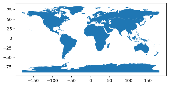
Suppose we are interested in studying continents, but we only have country-level data like the country dataset included in geopandas. We can easily convert this to a continent-level dataset.

Note

See also https://geopandas.org/en/stable/docs/user_guide/aggregation_with_dissolve.html

world = gpd.read_file("https://naciscdn.org/naturalearth/110m/cultural/ne_110m_admin_0_countries.zip")

world.head(3)

	featurecla	scalerank	LABELRANK	SOVEREIGNT	SOV_A3	ADM0_DIF	LEVEL	TYPE	TLC	ADMIN	...	FCLASS_TR	FCLASS_ID	FCLASS_PL	FCLASS_GR	FCLASS_IT	FCLASS_NL	FCLASS_SE	FCLASS_BD	FCLASS_UA	geometry
0	Admin-0 country	1	6	Fiji	FJI	0	2	Sovereign country	1	Fiji	...	None	None	None	None	None	None	None	None	None	MULTIPOLYGON (((180 -16.06713, 180 -16.55522, ...
1	Admin-0 country	1	3	United Republic of Tanzania	TZA	0	2	Sovereign country	1	United Republic of Tanzania	...	None	None	None	None	None	None	None	None	None	POLYGON ((33.90371 -0.95, 34.07262 -1.05982, 3...
2	Admin-0 country	1	7	Western Sahara	SAH	0	2	Indeterminate	1	Western Sahara	...	Unrecognized	Unrecognized	Unrecognized	None	None	Unrecognized	None	None	None	POLYGON ((-8.66559 27.65643, -8.66512 27.58948...

3 rows × 169 columns

world

	featurecla	scalerank	LABELRANK	SOVEREIGNT	SOV_A3	ADM0_DIF	LEVEL	TYPE	TLC	ADMIN	...	FCLASS_TR	FCLASS_ID	FCLASS_PL	FCLASS_GR	FCLASS_IT	FCLASS_NL	FCLASS_SE	FCLASS_BD	FCLASS_UA	geometry
0	Admin-0 country	1	6	Fiji	FJI	0	2	Sovereign country	1	Fiji	...	None	None	None	None	None	None	None	None	None	MULTIPOLYGON (((180 -16.06713, 180 -16.55522, ...
1	Admin-0 country	1	3	United Republic of Tanzania	TZA	0	2	Sovereign country	1	United Republic of Tanzania	...	None	None	None	None	None	None	None	None	None	POLYGON ((33.90371 -0.95, 34.07262 -1.05982, 3...
2	Admin-0 country	1	7	Western Sahara	SAH	0	2	Indeterminate	1	Western Sahara	...	Unrecognized	Unrecognized	Unrecognized	None	None	Unrecognized	None	None	None	POLYGON ((-8.66559 27.65643, -8.66512 27.58948...
3	Admin-0 country	1	2	Canada	CAN	0	2	Sovereign country	1	Canada	...	None	None	None	None	None	None	None	None	None	MULTIPOLYGON (((-122.84 49, -122.97421 49.0025...
4	Admin-0 country	1	2	United States of America	US1	1	2	Country	1	United States of America	...	None	None	None	None	None	None	None	None	None	MULTIPOLYGON (((-122.84 49, -120 49, -117.0312...
...	...	...	...	...	...	...	...	...	...	...	...	...	...	...	...	...	...	...	...	...	...
172	Admin-0 country	1	5	Republic of Serbia	SRB	0	2	Sovereign country	1	Republic of Serbia	...	None	None	None	None	None	None	None	None	None	POLYGON ((18.82982 45.90887, 18.82984 45.90888...
173	Admin-0 country	1	6	Montenegro	MNE	0	2	Sovereign country	1	Montenegro	...	None	None	None	None	None	None	None	None	None	POLYGON ((20.0707 42.58863, 19.80161 42.50009,...
174	Admin-0 country	1	6	Kosovo	KOS	0	2	Disputed	1	Kosovo	...	Admin-0 country	Unrecognized	Admin-0 country	Unrecognized	Admin-0 country	Admin-0 country	Admin-0 country	Admin-0 country	Unrecognized	POLYGON ((20.59025 41.85541, 20.52295 42.21787...
175	Admin-0 country	1	5	Trinidad and Tobago	TTO	0	2	Sovereign country	1	Trinidad and Tobago	...	None	None	None	None	None	None	None	None	None	POLYGON ((-61.68 10.76, -61.105 10.89, -60.895...
176	Admin-0 country	1	3	South Sudan	SDS	0	2	Sovereign country	1	South Sudan	...	None	None	None	None	None	None	None	None	None	POLYGON ((30.83385 3.50917, 29.9535 4.1737, 29...

177 rows × 169 columns

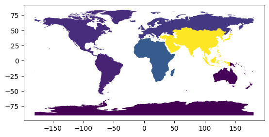
continents = world.dissolve(by="CONTINENT").geometry

continents.plot();

If we are interested in the population per continent, we can pass different aggregation strategies to the dissolve() functionusing the aggfunc argument:

https://geopandas.org/en/stable/docs/user_guide/aggregation_with_dissolve.html#dissolve-arguments

continents = world.dissolve(by="CONTINENT", aggfunc=dict(POP_EST="sum"))

continents.plot(column="POP_EST");

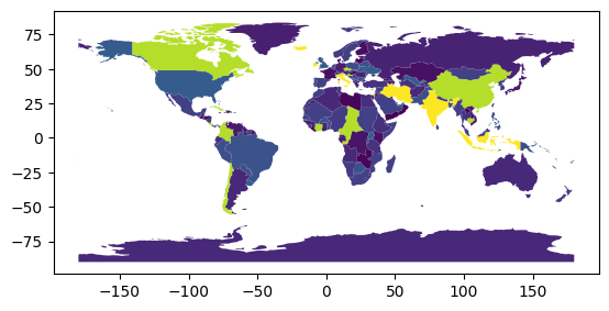
You can also pass a pandas.Series to the dissolve() function that describes your mapping for more exotic aggregation strategies (e.g. by first letter of the country name):

world.dissolve(by=world.NAME.str[0], aggfunc=dict(POP_EST="sum")).plot(column="POP_EST")

<Axes: >

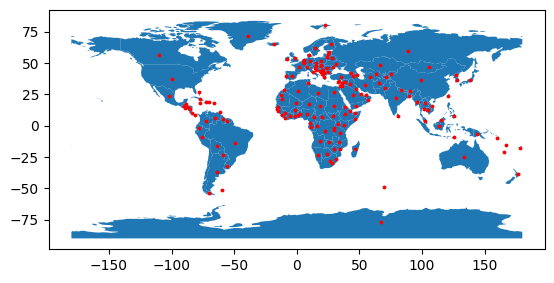
Representative Points and Crow-Fly Distances

The following example includes code to retrieve representative points from polygons and to calculate the distance on a sphere between two points.

Note

See also https://en.wikipedia.org/wiki/Haversine_formula

See also https://geopandas.org/en/stable/docs/reference/api/geopandas.GeoSeries.distance.html

world = gpd.read_file("https://naciscdn.org/naturalearth/110m/cultural/ne_110m_admin_0_countries.zip")

points = world.representative_point()

fig, ax = plt.subplots()
world.plot(ax=ax)
points.plot(ax=ax, color="red", markersize=3);

points = points.to_crs(4087)
points.index = world.ISO_A3

distances = pd.concat({k: points.distance(p) for k, p in points.items()}, axis=1).div(
    1e3
)  # km

distances.loc["DEU", "NLD"]

564.4945392494385

Global Equal-Area and Equal-Distance CRS

Previously, we used EPSG:3035 as projection to calculate the area of regions in km². However, this projection is not correct for regions outside of Europe, so that we need to pick different, more suitable projections for calculating areas and distances between regions.

• for calculating distances: WGS 84 / World Equidistant Cylindrical (EPSG:4087)

• for calculating areas: Mollweide (ESRI:54009)

The unit of measurement for both projections is metres.

AREA_CRS = "ESRI:54009"
DISTANCE_CRS = "EPSG:4087"

world = gpd.read_file("https://naciscdn.org/naturalearth/110m/cultural/ne_110m_admin_0_countries.zip")

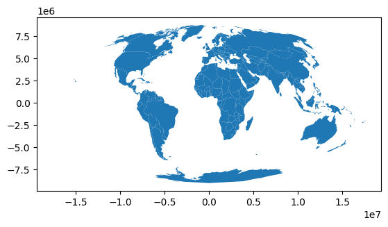
world.to_crs(AREA_CRS).plot()

<Axes: >

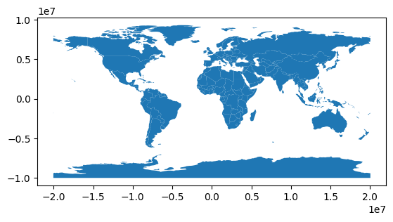
world.to_crs(DISTANCE_CRS).plot()

<Axes: >

Country Converter

The country converter (coco) is a Python package to convert and match country names between different classifications and between different naming versions.

Note

See also konstantinstadler/country_converter

import country_converter as coco

Convert various country names to some standard names, specifying source and target classification scheme:

coco.convert(names="NLD", to="name_official")

'Kingdom of the Netherlands'

coco.convert(names="NLD", to="iso2")

'NL'

coco.convert(names="NLD", src="iso3", to="iso2")

'NL'

country_list = ["AE", "AL", "AM", "AO", "AR"]

coco.convert(names=country_list, src="iso2", to="short_name")

['United Arab Emirates', 'Albania', 'Armenia', 'Angola', 'Argentina']

List of included country classification schemes:

cc = coco.CountryConverter()
cc.valid_country_classifications

['DACcode',
 'Eora',
 'FAOcode',
 'GBDcode',
 'GEOnumeric',
 'GWcode',
 'IOC',
 'ISO2',
 'ISO3',
 'ISOnumeric',
 'UNcode',
 'ccTLD',
 'name_official',
 'name_short',
 'regex']

Gurobi

Gurobi is one of the most powerful solvers to solve optimisation problems. It is a commercial solver, with free academic licenses.

Note

Using this solver for the group assignment is optional. You can also use other open-source alternatives, but they might just take a little longer to solve.

To set up Gurobi, you need to:

• Register at https://pages.gurobi.com/registration/ with your institutional e-mail address (e.g. @campus.tu-berlin.de).

• Follow the getting started guide for your respective operating system at https://www.gurobi.com/documentation/quickstart.html (this includes a guide for retrieving your academic license and installing the software).

• In your conda environment, install gurobipy with pip install gurobipy.